-
Graphing Linear Equations and Inequalities
At its most basic level, a linear equation is a function with variables and constants. These variables include x, y, or often times both.
There are a handful of ways to write linear equations:
- Point-slope form
- Slope-intercept form
- Standard form
The type of form determines how you graph the linear equation and determine its x and y-intercepts.
However, we can graph more than linear equations. We can also graph linear inequalities.
A linear inequality is simply a linear equation that doesn’t have an equal sign. Instead, it has one of the following symbols:
- Greater than (>)
- Less than (<)
- Greater than or equal to (≥)
- Less than or equal to (≤) symbol
Here, we will be explaining the many forms of linear equations and inequalities, and showing you how to graph them. Graphing a linear function allows you to find various combinations of points that, when plugged in, serve as a solution to the equation.
Let’s start by learning how to graph a linear equation in point-slope form…
Point-Slope Form
The point-slope form of a linear equation is written as y − y1 = m(x − x1). The values of x1 and y1 represent a specific point on the graph, and m represents the slope of the equation. This form is used when we only know one set of points and want to determine additional points by using the slope of the equation.
Here is an example of a linear equation in point-slope form:
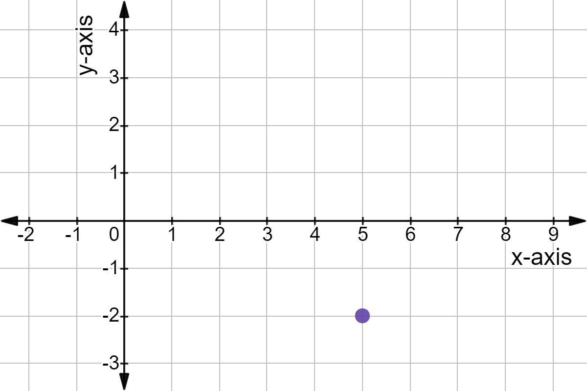
y+2 = 3/2 (x−5)
Note that anytime a set of points is in point-slope form, any positive sign in front of the values of x1 and y1 must be reversed to negative and any negative sign must be reversed to positive. So for this equation, x1= -2 and y1=5. Let’s graph this point accordingly:
Now let’s use the slope of this equation to determine the next point. Because the slope is 3/2, let’s move the y-value in the positive direction (upward) by three points and shift the x-value in the positive direction (to the right) two points:
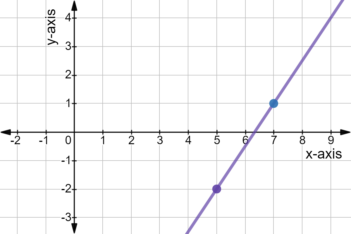
By moving point (5, -2) up three spaces and right two, we’ve determined that the next point on the graph is (7,1.)
Now that we’ve learned Point-Slope Form, let’s review the slope-intercept form of a linear equation…
Slope-Intercept Form
Slope-intercept form is the most common way to write a linear equation. It uses the formula
y = mx + b.
In this form, m represents the slope of the line and b represents the y-intercept. This form makes it really easy to plug in x-values to determine their correlating y-values, and vice versa. Here is an example of a linear equation in slope-intercept form:
y = 4/3x + 2
Let’s determine the x-intercept by plugging in zero for y:
y = 4/3x + 2
(0) = 4/3x + 2
-2 = 4/3x
3/4(-2) = x
–64 = x
x − intercept = -1.5
We’ve now determined that the x-intercept for this equation is (-1.5, 0.)
Now that we’ve reviewed point-slope form, let’s learn how to write a linear equation in standard form…
Standard Form
Standard form is a way of displaying linear functions with the x and y values on the same side of the equation:
Ax + By = C.
The rules of standard form are that the values of A, B, and C must all be whole numbers with no fractions or decimals. Additionally, the value of A must always be positive.
Here is an example of an equation written in standard form:
2x − 3y = 6
This form makes it easy to write find the x and y-intercepts, all you have to do is plug in zero:
2x − 3(0 = 6
2x = 6
x = 6/2
x − intercept = (3,0)
2(0) − 3y = 6
-3y = 6
y = –6/3
y − intercept = (0, -2)
How to Graph Linear Inequalities
Graphing linear inequalities uses all the same steps as graphing a linear equation. The big difference is that linear inequalities use greater than (>), less than (<), greater than or equal to (≥), and less than or equal to (≤) symbols instead of an equal sign. Because of this, additional steps must be taken when graphing a linear inequality.
When graphing an inequality, you must decide whether to use a dotted or solid line for the linear equation. You must also shade either the section left or right of the graphed line depending on each given inequality statement.
Let’s explain how to take these additional steps for graphing a linear inequality…
Step 1: Arrange Inequality into Slope-Intercept Form
When you’re working with a linear inequality, you ought to have y on its own side of the equation, separate from other numbers and variables. This means that we must convert linear inequalities into slope-intercept form. Here’s an example:
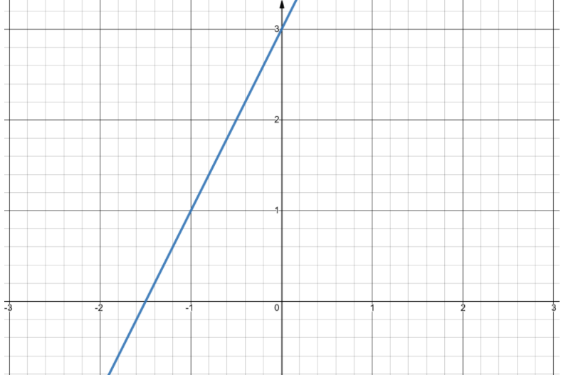
y – 3 > 2x
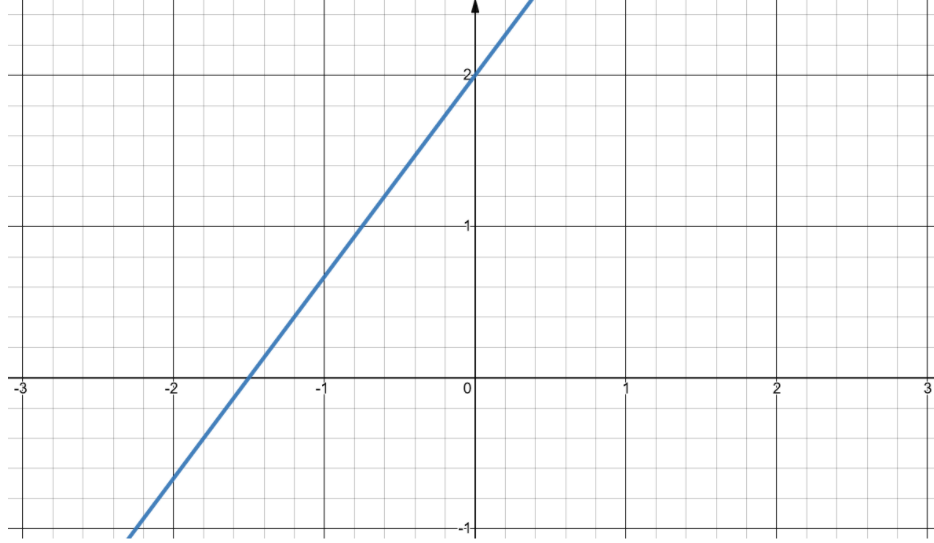
y > 2x +3
Now that the equation is in slope-intercept form, graph it just like a regular linear equation:
Step 2: Determining Strict Inequalities
Now that we have the equation graphed, we must decide whether it’s a strict inequality or not. Determining this will tell us if we should use a solid or dashed boundary line. A boundary line separates the graph into two sections and shows us which points can serve as possible solutions to the inequality.
A strict linear inequality has a “>” or “<” sign. In these inequalities you’ll use a dashed line to indicate that any points on this line cannot be possible solutions to the inequality.
A non-strict inequality has a “≥” or “≤” sign. For these inequalities, you’ll use a solid line to indicate that any set of points along this line can be a possible solution to the inequality equation. When you plug in any x or y values on this line, the linear inequality equation will still be true.
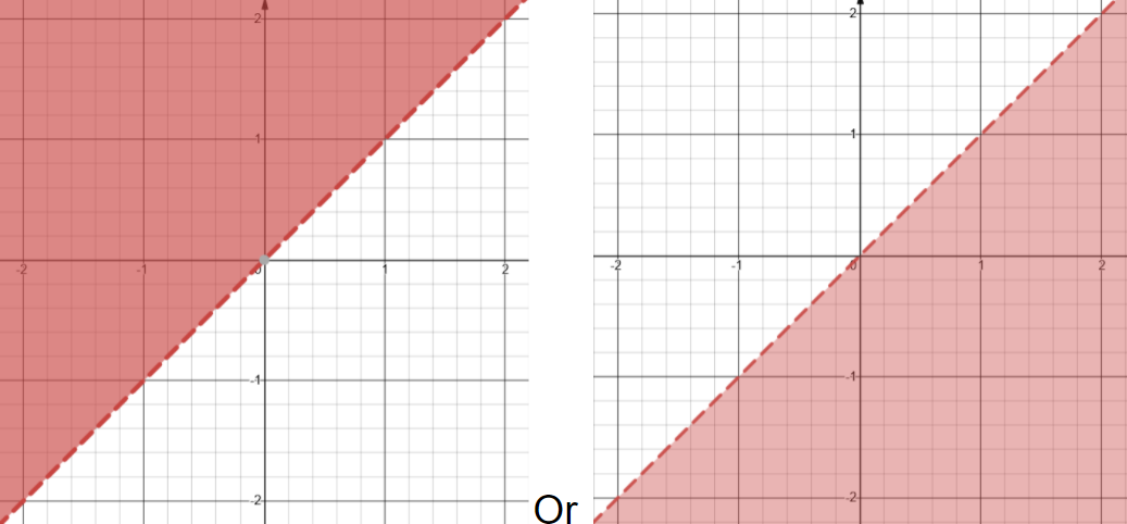
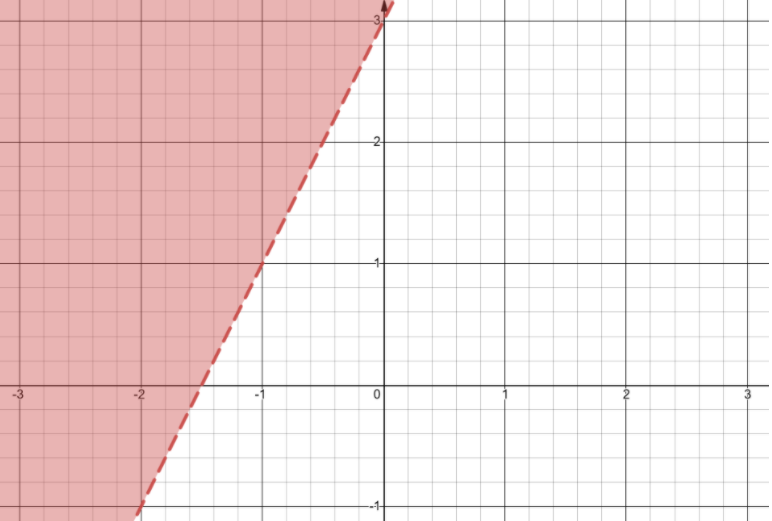
The equation y > 2x + 3 is a strict inequality so let’s use a dotted line to graph it:

Step 3: Deciding the Shaded Region
The last step for graphing linear inequalities is choosing which side of the boundary line you need to shade. This shaded area will incorporate every point that satisfies the inequality.
The best way to determine the shaded side is to select a testing point like (0,0) and plug it into the inequality. If plugging in this point makes the inequality true, shade the side of the graph that point lies on. If the testing point makes the inequality untrue, shade the other side of the graph.
Lets plug (0,0) into the equation y > 2x + 3:
(0) > 2(0) + 3
0 > 3
This equation is clearly untrue as 0 is not greater than 3. Because of this, we will shade the left side of the dotted line on our graph:
Still struggling to understand linear equations and inequalities? We don’t blame you! Algebra is a tough subject and many of us need extra help to master it.
That’s where Tutor Portland comes in. We provide students with tutors who specialize in algebra along with numerous other math subjects. Our tutors give you the one-on-one support you need to keep up with homework and score high on exams. Whether you want in-home or virtual sessions, Tutor Portland will find the perfect tutor to help you with concepts like Linear Equations and Inequalities. Sign up today for a free intro session!